Continuous charge distribution
NCERT Class 12 Physics Chapter 1 Section 1.12
Quick answer
A continuous charge distribution is charge spread along a wire, over a surface or through a volume, described by a charge density: λ = ΔQ/Δl in C/m, σ = ΔQ/ΔS in C/m and ρ = ΔQ/ΔV in C/m. Each element is small on the everyday scale but holds very many charges, so the density is a smoothed-out average that ignores quantisation. The field is found by treating each element as a point charge and adding their fields by superposition.
With your textbook
NCERT Physics Part I (Class 12), Chapter 1 “Electric Charges and Fields”, Section 1.12 “Continuous Charge Distribution”, pages 28–29.
Open the official NCERT chapter (PDF, 4.0 MB, ncert.nic.in) (opens in a new tab)
Checked against the 2026-27 reprint on .
What is a continuous charge distribution?
Continuous charge distribution
Charge spread along a wire, over a surface or through a volume is described by a charge density: the charge per unit length, area or volume. NCERT sums up why this works:
In short, using Coulomb’s law and the superposition principle, electric field can be determined for any charge distribution, discrete or continuous or part discrete and part continuous.
NCERT Physics Part I (Class 12), Section 1.12, page 29
In plain words: a charged metal surface holds billions upon billions of electrons, and nobody can list where each one sits. So we zoom out: cut the surface into patches that are tiny to us but still hold huge numbers of charges, and say how much charge each patch carries per square metre. That smoothed-out number is the surface charge density.
Linear, surface and volume charge densities
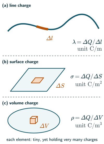
Working with discrete charges is simpler and needs no calculus, but for many purposes it is impractical: on the surface of a charged conductor, for example, we cannot specify where each microscopic charge sits (NCERT page 28). Instead we take elements that are small on the macroscopic scale but large enough to hold a very large number of charges (page 28):
Charge densities (NCERT Eqs. 1.23–1.25)
- Surface charge density σ: the charge ΔQ on an area element ΔS; unit C/m2 (NCERT Eq. (1.23), page 28).
- Linear charge density λ: the charge on a short line element Δl of a wire; unit C/m (NCERT Eq. (1.24), page 28).
- Volume charge density ρ, sometimes simply called the charge density: the charge in a volume element ΔV; unit C/m3 (NCERT Eq. (1.25), page 28).
- These densities are macroscopic: a smoothed-out average over an element that is large microscopically but small macroscopically. They ignore the quantisation of charge and the gaps between charges at the microscopic level (pages 28–29).
- It is the same idea as the density of a liquid: we treat the liquid as a continuous fluid and ignore its molecules (NCERT page 29). Compare density of a fluid, ρ = m/V.
Field of a continuous charge distribution
The field is found as for discrete charges (NCERT Eq. (1.10)), one small element at a time (page 29):
- Divide the distribution into small volume elements ΔV. The charge in each is ρΔV, where ρ may vary from point to point.
- Each element acts like a point charge. At a point P, inside or outside the distribution, its field is given by Coulomb’s law (NCERT Eq. (1.26)):
Field of one element (NCERT Eq. 1.26)
Here k = 1/4πε0, r′ is the distance from the element to P and r̂′ is the unit vector from the element towards P.
- By superposition, the total field is the sum over all the elements (NCERT Eq. (1.27), page 29):
Total field (NCERT Eq. 1.27)
- Strictly, ΔV → 0 and the sum becomes an integral; NCERT leaves that out for simplicity (page 29). The same steps work with λΔl for a line and σΔS for a surface.
Solved examples
Example 1: Charge densities
(a) A thin rod 0.50 m long carries 2.0 µC spread evenly. (b) An isolated metal sphere with no external field, of radius 0.10 m, carries 1.0 × 10⁻⁸ C on its surface. Find λ and σ.
Answer: (a) λ = Q/l = (2.0 × 10⁻⁶)/0.50 = 4.0 × 10⁻⁶ C/m. (b) The surface area is 4πR2 = 4π(0.10)2 ≈ 0.1257 m2, so
(NCERT Eqs. (1.23) and (1.24), page 28.)
Example 2: Charge on a large sphere (NCERT Exercise 1.21(a))
A uniformly charged conducting sphere of diameter 2.4 m has a surface charge density of 80.0 µC/m2. Find the charge on the sphere.
Answer: R = 1.2 m, so the area is 4πR2 = 4π(1.2)2 ≈ 18.1 m2, and
(NCERT Eq. (1.23), page 28; the flux through this sphere is found on the Gauss’s law page.)
Example 3: Charge in a charged ball
A ball of radius 5.0 cm has a uniform volume charge density of 2.0 × 10⁻⁵ C/m3. Find its charge.
Answer: the volume is (4/3)πR3 = (4/3)π(0.050)3 ≈ 5.24 × 10⁻⁴ m3, so Q = ρV ≈ (2.0 × 10⁻⁵)(5.24 × 10⁻⁴) ≈ 1.0 × 10⁻⁸ C (NCERT Eq. (1.25), page 28).
Example 4: Field on the axis of a charged ring
A thin ring of radius R carries a charge Q spread evenly. Find the field at a point P on its axis, a distance x from the centre.
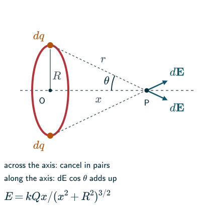
Answer: use NCERT’s method (Eq. (1.27), page 29) with small elements dq of the ring. Every element is the same distance r = √(x2 + R2) from P, and gives a field k dq/r2 along the line from it to P.
- For each element there is one diametrically opposite. Their field parts across the axis cancel.
- Their parts along the axis add: each is k dq/r2 × cos θ, with cos θ = x/r.
Adding over the whole ring, the dq add up to Q:
directed along the axis, away from the ring for positive Q. Checks: at the centre, x = 0 and E = 0, as symmetry demands; far away, x ≫ R and E ≈ kQ/x2, the field of a point charge.
Common mistakes to avoid
Common mistake
Mixing up the three densities
λ is charge per length (C/m), σ per area (C/m) and ρ per volume (C/m). Check the unit before you multiply (NCERT page 28).
Common mistake
Thinking a density means the charge is truly smooth
The densities are macroscopic averages; at the microscopic level charge is in discrete lumps with empty space between (NCERT pages 28–29).
Common mistake
Adding the fields of elements as plain numbers
Each element’s field has its own direction, so the fields add as vectors; symmetry often makes some parts cancel, as across the axis of a ring (NCERT page 29).
Quick revision summary
- Continuous distributions are described by charge densities over elements that are small macroscopically but hold very many charges.
- σ = ΔQ/ΔS (C/m), λ = ΔQ/Δl (C/m), ρ = ΔQ/ΔV (C/m): smoothed-out macroscopic averages that ignore quantisation.
- Field: treat each element as a point charge, ΔE = k ρΔV/r′ along r̂′, and add by superposition; exactly, the sum becomes an integral.
- Coulomb’s law with superposition gives the field of any charge distribution, discrete, continuous or mixed.
- Charged ring, on its axis: E = kQx/(x + R)^(3/2), zero at the centre, like a point charge far away.
Formula sheet
- λ = ΔQ/Δl (C/m)
- σ = ΔQ/ΔS (C/m)
- ρ = ΔQ/ΔV (C/m)
- ΔE = k ρΔV/r′, along r̂′
- E ≈ Σ k ρΔV/r′ r̂′
Questions students ask
What is the difference between discrete and continuous charge distribution?
A discrete charge distribution is a set of separate point charges, whose fields are added one by one, while a continuous charge distribution is charge spread along a line, over a surface or through a volume, described by a charge density, whose field is added up element by element (NCERT pages 28–29). The difference is one of scale: all charge is discrete at the microscopic level, but a charged body holds so many electrons that a smooth density is the practical description (NCERT page 28). One practical difference: the field of point charges is not defined at the charges themselves, while a bounded, sufficiently regular volume charge density gives a finite field inside it too; this does not extend automatically to singular ideal line or surface distributions (NCERT page 41).
What are the dimensional formulae of linear, surface and volume charge density?
The linear, surface and volume charge densities, λ, σ and ρ, have the dimensional formulae [L T A], [L T A] and [L T A], with SI units C m, C m and C m (NCERT page 40). Each is a charge, with dimensions [A T], divided by a length, an area or a volume (see dimensional formulae). Like the charge itself, a density can be positive or negative.
Has continuous charge distribution been deleted from NCERT and the JEE and NEET syllabus?
No, continuous charge distribution is still part of the course: it is in NCERT Class 12 Physics Part I as Section 1.12 (pages 28–29 of the 2026–27 reprint). The JEE Main syllabus lists it in Unit 11, Electrostatics: “forces between multiple charges, superposition principle and continuous charge distribution”, and the NEET (UG) 2026 syllabus names it in the same place in its Unit 11. The topic covers the three densities, λ, σ and ρ, and finding a field by adding the fields of small elements (NCERT pages 28–29).
What is the electric field at the centre of a uniformly charged semicircular ring?
The field at the centre of a thin semicircular ring of radius R with charge Q spread evenly is E = 2kλ/R = 2kQ/(πR), where λ = Q/(πR), directed along the ring’s line of symmetry, away from the ring for positive Q (beyond the NCERT text, by NCERT’s method of adding the fields of small elements, page 29). Every element is the same distance R from the centre; the parts of the fields across the symmetry line cancel in pairs, and the parts along it add up to twice kλ/R. A full ring gives zero at its centre, because its two halves cancel.
Practice questions
Try each question first, then open the answer to check your working.
-
Q1. Give the SI units of linear, surface and volume charge density.
Show answerHide answer
C/m, C/m2 and C/m3 (NCERT page 28).
-
Q2. A plate of area 0.2 m carries 4 × 10 C spread evenly on one face. Find σ.
Show answerHide answer
σ = Q/A = (4 × 10⁻⁹)/0.2 = 2 × 10⁻⁸ C/m2 (NCERT Eq. (1.23), page 28).
-
Q3. Why can a charge density ignore the quantisation of charge?
Show answerHide answer
Because each element, though small on the everyday scale, holds a very large number of charges, so the density is a smoothed-out average (NCERT page 28).